TRN User's Guide
Introduction
TRN is an algorithm that produces a best estimate of a vehicle’s position by combining a dead-reckoned measurement of its motion (e.g. velocities from a DVL or AHRS) with measured ranges to the seafloor (e.g. from a DVL, multibeam sonar, atlitmeter, etc). Specifically, the goal of the algorithm is to estimate at every time step the Northings, Eastings and Depth (NED) position of the vehicle with respect to a bathymetry map stored on-board. That is, the vehicle’s position is localized with respect to the terrain, not to GPS coordinates. Importantly, the goal also includes estimating the confidence in that position (covariance). This metric provides a means of determining whether the TRN position estimate should be accepted by the vehicle’s navigation and control system.
To accomplish this, the TRN algorithm employs a Particle Filter (PF) implementation of an Extended Kalman Filter (EKF). An EKF is required because the equations used to propagate the estimate are nonlinear. A PF implementation is chosen for several reasons. One is that the convergence of EKFs is known to be highly dependent on the accuracy of the initial estimate, and this is problematic for many field applications. Initial estimates can be off by hundreds of meters or more, for example due to a long descent from the surface with no bottom lock and hence poor navigation. Another is that the contours in the terrain can be similar at multiple locations, which creates multiple possible potential solutions for the algorithm to consider.
The core of the EKF and the PF is an iterative two-step process. First is a Process Update (or Position Update). Second is a Measurement Update. In the Process Update, the equations of motion for the vehicle are propagated from one time step to the next. This is typically done by integrating the measured velocity (e.g. from a DVL or IMU) or accepting a delta-position change from an INS. In the Measurement Update, range measurements from an acoustic device (e.g. DVL, altimeter, multibeam, etc.) are compared to range measurements calculated from the estimated vehicle location in the bathymetry map. The errors in these range measurements provide the innovations that are used to generate corrections to the vehicle position calculated in the Motion Update.
The difference between an EKF and a PF is that the EKF propagates these steps using known equations, and the PF uses a numerical, Monte-Carlo approach. Specifically, the PF propagates multiple (e.g. 10,000 or more) hypothesized locations of the vehicle (particles) plus weightings on each particle that quantify how well the predicted range measurements match the measured ranges. The PF implementation results will match the EKF equation results exactly when the number of particles goes to infinity.
TRN can be run real-time or as a post processing aid. When run in real time, the best estimates of the vehicle’s position provided by TRN can be used to correct the navigation data used by the control system. This eliminates drift errors typical of most onboard dead reckoning navigation algorithms (e.g. DVL based AHRS) as well as any georeferencing errors in the bathymetry. An example of a mission enabled by TRN is returning to a site of interest (indicated as a point on a map) without using any external infrastructure. Acoustic arrays, beacons or surface aiding navigation aids are not required.
The navigation accuracy provided by TRN is typically on the same order of magnitude as the resolution of the bathymetry map being used. In work using 1m maps, TRN accuracy of 2 to 3m meters is typically seen.
TRN is meant to be used to provide a correction to the navigation data in closed-loop applications. It is not intended as the sole navigation solution. The reason is that navigation loops are often closed at high sample rate (e.g. 0.4seconds) and the sample rate of TRN is typically slow (e.g. 4 seconds). One reason for this slow rate is that a PF implementation of TRN is computationally expensive. Another critical reason is that a slow rate is required to ensure that all the measurement data entering the TRN algorithm is uncorrelated.
II. Sample Mission:
Before describing how TRN operates, a description of the output produced by TRN can be demonstrated using a sample mission performed at Portuguese Ledge by an LRAUV equipped with a DVL. The map used for this mission had a resolution of 1m. The vehicle’s navigation system used the DVL, compass and attitude sensors (pitch and roll) to calculate a dead-reckoned solution. This type of system is called an AHRS (Attituded Heading Reference System). The vehicle’s control logic included an integral loop which forced the error between the AHRS solution and the commanded path to go to zero.
The goal of this mission was to fly a trajectory consisting of straight lines between four waypoints specified on a bathymetry map. This mission was flown twice. In the first run, the path was flown using the unaided, baseline navigation system on board the vehicle. In the second, the navigation solution was corrected with the TRN algorithm. In each mission, the vehicle made two passes around loop.
The resulting path for the first run is shown in Figure 1. The target waypoints are shown as red stars. The black line in the figure is the recorded AHRS path. The blue line is the best estimate of the true path provided by TRN. The path starts just above the Eastern most waypoint and ends with the AUV approaching that same waypoint from the Northeast.
As can be seen in the figure, the AHRS estimate of the path converges to a sequence of straight lines connecting the waypoints as expected. However, this path exhibits significant error as shown by the blue TRN path.
There are several reasons for this error. First is that the map used in this case is known to have georeferencing errors (approximately 20m), so an offset is expected. Second, the offset is large because a dead-reckoning error had accumulated as the vehicle approached the start of the mission. This often occurs if the vehicle has suffered poor navigational performance while the DVL was out of contact with the seafloor (e.g. during a spiral down maneuver from the surface). Finally, there is a drift in the AHRS navigation which is common for any dead-reckoned solution and can be caused by uncertainties in the measured velocities as well as slight misalignments in the compass, DVL and attitude measurements.
Figure 2 plots the second important quantity provided by TRN. This is the confidence the TRN algorithm has in its best estimate of the vehicles position. Plotted is the covariance of the estimate (square of the standard deviation) for both the Northings (blue) and Eastings (black) estimates. As shown, these covariances hover between about 1 and 4 m^2 (i.e. standard deviation of 1 to 2m) except for a section of the path near the middle of the mission where the uncertainty spikes.
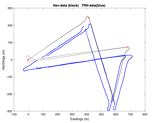
Fig 1: NED path between 4 waypoints (red *). AHRS data (black). TRN data (blue)
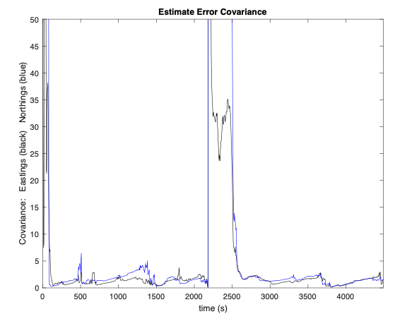
Fig 2: Covariance of the Eastings (black) and Northings (blue) TRN estimate of the TRN
The results for the second run are shown in Figure 3. In this case, the path used to control the vehicle incorporated the corrections provided by TRN. There are two curves in this figure. The blue curve is the TRN solution. The black curve is the corrected navigation data. Again, the navigation error is driven to zero by the integrator and the true path now matches the desired path. These curves overlap. (The nav data are updated every 0.4 seconds. The TRN data are updated every 4 seconds.)
The important thing to note is that the initial condition errors, the map georeferencing errors and the dead-reckoned drift have all been eliminated in the vehicle’s navigation data. The vehicle accurately follows the desired path.
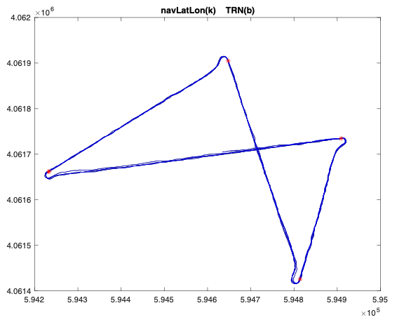
Fig 3: NED path between 4 waypoints (red *). AHRS data with TRN correction (black). TRN data (blue)
The only caveat to note is that the TRN estimate is a best estimate of the path, not necessarily the true path. This is a stochastic system, and the quality of the estimate depends on the noise and uncertainty in the data.
The parameters that describe this uncertainty and guidance on how to choose them are provided below. To begin, the basic operation of the Particle Filter used in the TRN algorithm is presented.
Summary of PF operation
As stated above, a particle filter operates by propagating a large number (e.g. 10,000 or more) hypothesized positions of the vehicle. Each particle consists of a Northings value, an Eastings value and a depth value. At every time step, beams are projected from each particle and their lengths are calculated (e.g. where the beam hits the bathymetery map).
This requires knowledge (i.e. configuration parameters) of the beam orientations with respect to the vehicle and measured values of the vehicle’s orientation (roll, pitch and yaw). How well the beam lengths match the measured beam lengths provides a metric of how likely each particle’s NED values correspond to the correct location of the vehicle.
The process (or motion) update performs the first step in this procedure. It calculates the motion of the vehicle between time steps and applies that motion to every particle. This can be done by integrating the equations of motion of the system or by measuring the change in position reported by the vehicle’s INS (the default mode in the TRN code). Random noise (a user defined input: dritRate) is then applied to each particle’s location. This sequence is depicted in Figure 4.
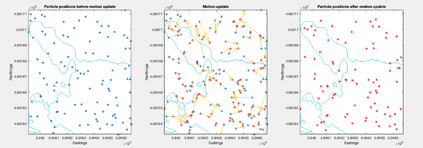
Fig 4: The Process Update: (a) particles before update, (b) delta motion and noise applied, (c) resulting particles
In the measurement update, the beam lengths associated with each particle are computed and a random noise is added (a user input: percentrangeerror). The resulting full set of particles with their associated weights defines the likelihood score for every hypothesized location.
Figure 5 depicts the data used in the measurement update to calculate the likelihood score for a particle. Shown is a sonar beam projected to a stored bathymetry map from a vehicle located at the particle’s position. The difference between the length of the measured beam and the distance to the map is the error in the measured range.
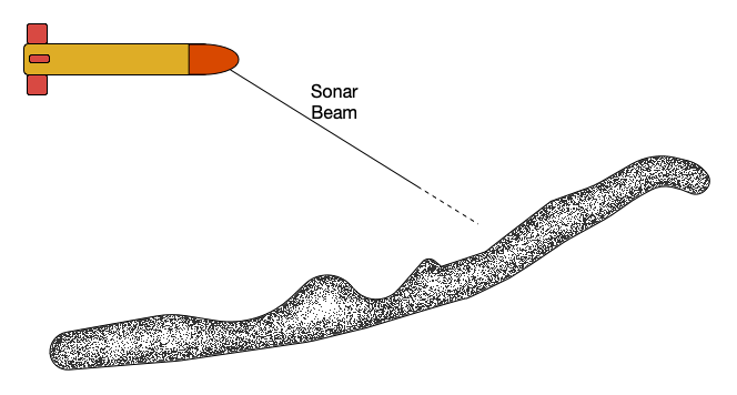
Fig 5: The Likelihood score is computed by comparing a meaured beam length to the distance to the terrain map.
If there is only one beam, the weight, \(w(i)\), assigned to each is calculated as
where the quantity \((l-l_m )\) is the error in the measured range, \(\sigma\) is the standard deviation of the measurement noise, and η is a normalizing coefficient. If there are multiple beams, the error is replaced by the sum over all the beams.
At any time step, the current best estimate of the vehicle position is the particle location where the weighted mean of the likelihood score is a maximum.
Ideally, the particles used in this iterative process would span the entire space of possible vehicle locations. Computationally this is not possible when the vehicle’s position is very uncertain, however. To overcome this, a particle filter computes a bounding box for the particles based on the current estimate of the filter’s confidence in the solution. The size of this box is adjusted dynamically to be (very roughly) 3 sigma in size using a “resampling” algorithm. This algorithm moves low-weight particles to higher weighted locations while preserving the probability distribution of the particle cloud.
An example is shown in Figure 6 for the example run provided above. The black line in the figure is the uncorrected navigation data. The bounding boxes are centered on the TRN solution (blue line).
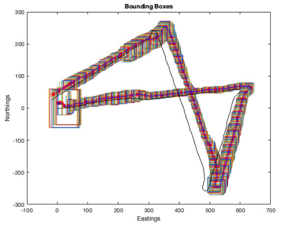
Fig 6: : Particle bounding boxes overlaid on TRN trajectory. Uncorrected AHRS data is the black line.
Figure 7 provides additional detail for the same example during a segment of the run where the PF was converging on a solution. Particle weights are plotted for five time points. The distribution of particle weights and the bounding box (red) are shown in the first column. The projections of the weights onto the Northings and Eastings directions are shown in the next two columns. The red vertical line in the location where the weighted average of the distribution is a maximum. The cyan line is the location of the peak in the distribution. As the filter converges to a solution, these two locations approach the same value.
This sequence presents one of the key advantages of using a PF implementation: a PF deals naturally with multimodal (i.e. existence of local minima) and non-Gaussian distributions. It propagates all possible solutions. The weights are reinforced or reduced as a mission continues until final convergence achieved. An EKF would likely fail to converge in this situation.
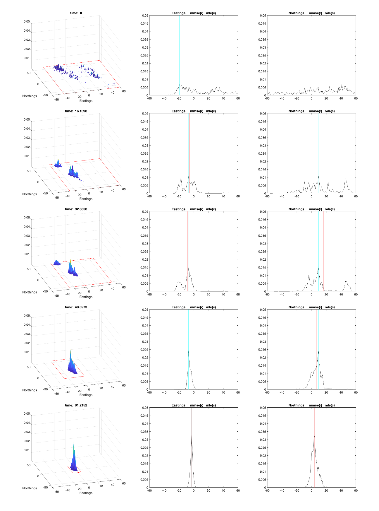
Fig 7: Sample results showing evolution of particle weights during TRN convergence. (a) partilce weights with bounding boxex, (b) weights vs.Eastings, (c) weights vs. Northings
Running TRN
Required inputs: motion data, range data and beam configuration data
The current version of TRN is configured to estimate three states: the Northings, Eastings and Depth positions of the vehicle. As described above, a measured time history of the motion inputs is required (e.g. AHRS NED values). For the measurement update, measured sonar ranges to the seafloor are required, for example DVL beam lengths, altimeter measurements or multibeam.
The motion update quantities are sampled simultaneously, and the update is typically at a constant rate, but a variable rate is acceptable.
In the measurement updates, every beam measurement is an independent input occurring at an asynchronous rate and can be treated separately. However, in practice, sonar devices often provide multiple beams simultaneously, and it is convenient to process these together using vector rather than scalar operations.
To be incorporated into the TRN solution, the configuration of every beam must be specified. This includes the location of the beam with respect to the origin of the vehicle’s reference frame (e.g. the compass) as well as its direction in the vehicle’s reference frame. Also required are measurements of the vehicle’s pitch, roll and yaw angles.
The details of how the beam data are specified and incorporated into the code are presented in SECTION: CODE DETAILS.
Required inputs: driftRate and \(percentagerangeerror\)
The PF used in the TRN algorithm, like all Kalman Filter type of estimators, is a stochastic system. It calculates a “best estimate” of the state (NED) given the inputs described above and estimates of the uncertainty in those measurements. The accuracy of these estimates depends on user defined values of the noise associated with the measurements that are used by TRN. TRN uses two variables for this purpose. The first, driftRate, describes the process (i.e. motion) noise. The second percentrangeerror defines the measurement noise.
Figure 8 demonstrates the stochastic nature of the TRN solution. Shown in the figure are 100 runs using the same input with a driftRate = 2% and \(percentagerangeerror\) = 2%. As can be seen, the TRN solution for each run is different (an expanded view of the spread is shown in Figure 9. In ideal cases, this spread is zero mean Gaussian centered about the true path.
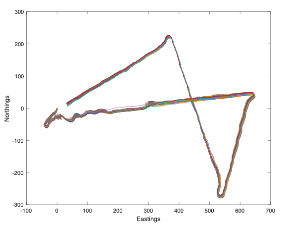
Fig 8: 100 runs for TRN for different noise values.
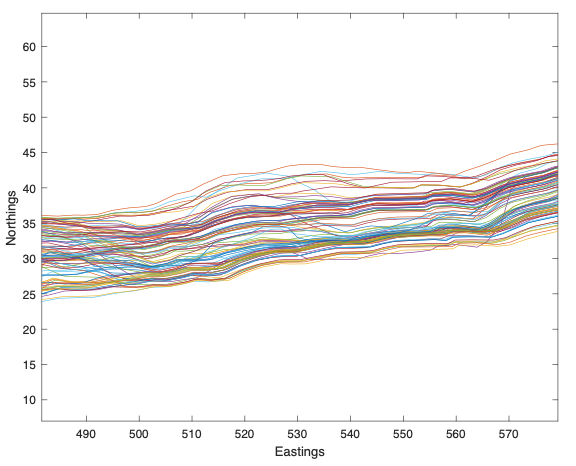
Fig 9: Expanded view of the 100 runs
The covariance (square of the standard deviation) of the state estimates (NED) produced by the TRN algorithm predicts the width of this spread. If the correct values of drfitRate and percentrangerror are chosen correctly (and all the zero-mean Gaussian noise assumptions are met), then, the width of the actual spread will match the covariance produced by the TRN, and the filter will be “consistent”.
Figure 10 and Figure 11 plot the time histories of all 100 runs of the Northings and Eastings estimates centered about the mean value at each time step. Also shown in the figure is the one sigma uncertainty bound produced by TRN (red). For a perfect choice of driftRate and percentrangeerror, roughly 63% of the curves will be inside this one sigma boundary.
NOTE: More properly, these curves would be plotted with one sigma bands on either side of the true values and not the mean values of the path. In practice however, the true path is often not known, and plots about the mean can be used. While this does provide a measure of validity of the noise parameters chosen, care must be taken when interpreting the reasonableness of the results. Looking at the smoothness of the mean is also necessary to determine the reasonableness of the result.
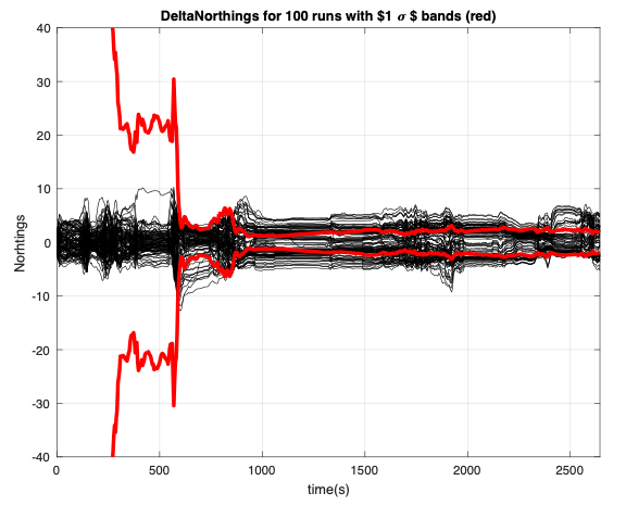
Fig 10: Northings values minus the mean for 100 runs (black). Mean standard deviation bound (red)
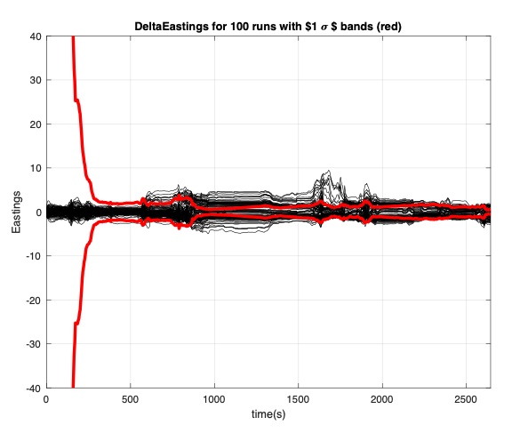
Fig 11: Eastings values minus the mean for 100 runs (black). Mean standard deviation bound (red)
To demonstrate the effect choosing different values of the noise parameters the TRN algorithm was run on sea trial data using an LRAUV using four different values of driftRate. Thes runs were done post dive 100 times each for driftRate values of 1%. 2%, 3% and 4% respectively. The percentrangeerror = 4% in all cases. The sonar beams used were the 4 beams of the onboard DVL.
The results are shown in Figure 12, Figure 13, Figure 14 and Figure 15. The standard deviations predicted by TRN along with the standard deviation of the 100 estimated trajectories is plotted vs. time for each case.
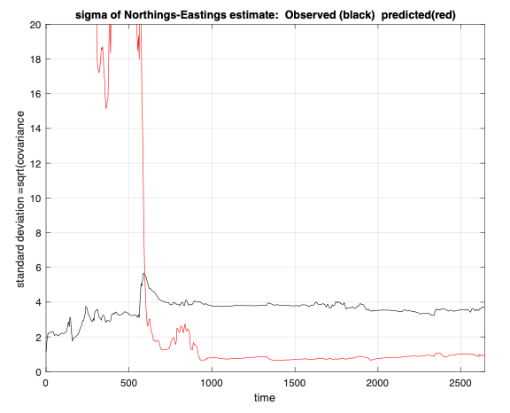
Fig 12: Standard deviation of NE position. Obaserved value (black). Predicted value (red). driftRate = 1%
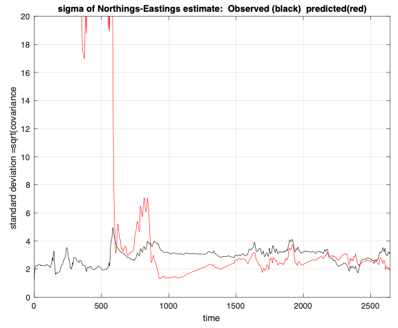
Fig 13: Standard deviation of NE position. Obaserved value (black). Predicted value (red). driftRate = 2%
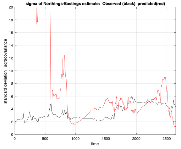
Fig 14: Standard deviation of NE position. Obaserved value (black). Predicted value (red). driftRate = 3%
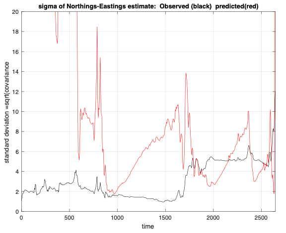
Fig 15: Standard deviation of NE position. Obaserved value (black). Predicted value (red). driftRate = 4%
Visible in the data is that the observed deviation of the width in trajectories (black line was approximately the same for all runs, but the value predicted by TRN depends on the user defined parameters. For the case driftRate = 1, it is clear that the predicted standard deviation is well below the observed value. It is also clear that for driftRate = 4, the predicted value is much larger. It is also evident that smaller values of the driftRate produce “tighter” converged solutions, even though the confidence in that solution is overly optimistic.
Choosing a driftRate = 2 would be a reasonable choice for this mission.
Choosing the number of beams
The examples presented above focused on the effect the two user defined parameters, driftRate and percentrange error, have on TRN performance. An additional degree of freedom in the system is the number of beams that are used in the measurement update. All of the above examples used the four beam lengths from the DVL (which also measured the vehicle’s velocity with respect to the seafloor). TRN can accept any number of beams. Clearly, using more beams offers more information. However, there are issues.
One obvious issue with increasing the number of beams is that beam ray tracing is computationally expensive and may affect the sample rate. Another issue is that TRN treats each beam as being completely uncorrelated from all the others. Any correlation results in information being “duplicated” with the result that the TRN filter will over converge, meaning that the estimates of the covariance uncertainties will be overly optimistic.
A common source of correlation is the beam soundings being too closely spaced. Overlapping of beam footprints is an obvious issue. Less obvious is that beam filtering techniques that use averages of beams adds correlation. Even less obvious is an assumption that the terrain is also assumed to be completely uncorrelated, meaning that knowing the terrain height at one location provides “no information” about the terrain height 1m away. The variations in real terrain do not meet this assumption, consequently larger spacing between beam soundings is good practice (a minimum of 3 or 4 meters has proven reasonable).
Choosing the noise and beam parameters
As described above, the user defined parameters that determine the performance of TRN are the driftRate, percentrangeerror and the number of beams. Often, these parameters are selected based on experience with using TRN at a site. For new missions, initial estimates can be obtained by testing multiple TRN configurations in simulation. Another option is to exploit the equivalence between a PF and an EKF. The advantage is that the EKF provides equations that provide insight into the sensitivity of algorithms performance with respect to parameter variations.
Sensitivity studies can be done using the EKF equations described in "Running TRN" below. A sample set of plots is presented in Figure 16, Figure 17 and Figure 18. Plotted are the standard deviations of the NED position as a function of the driftRate and percentrangeerror with 4 beams, 7 beams and 11beams. In each case the beams are pointed downwards in a cross-track configuration and are evenly spaced across a 90deg span. The standard deviation of the depth error for these plots was 0.5m. A trajectory at Portuguese Ledge as used as the baseline.
To generate these equations, the measurement matrix, H, was calculated along a nominal path in the terrain. Each element in H is the delta chance in beam length for a delta motion in either the Northings, Eastings or depth direction. Given H, the EKF covariance equations were iterated to steady-state at each time step.
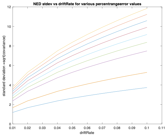
Fig 16: Predicted standard deviation of NE estimate using 4 besms.
percentrangeerror = [.01 .02 .02 .04 .05 .06 .07 .08 .09 .10]. MNM = 2
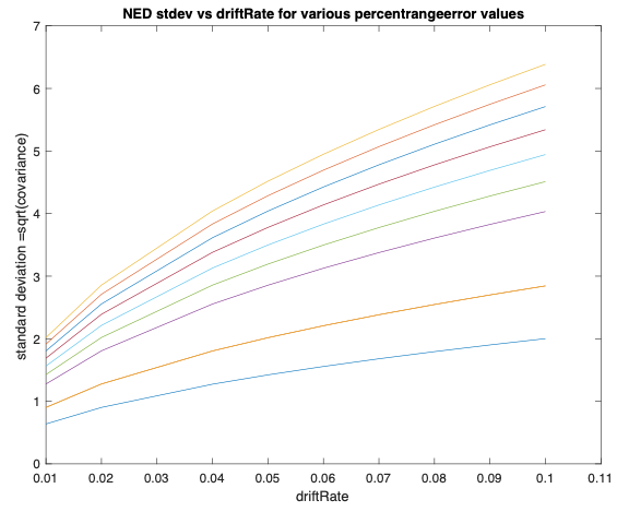
Fig 17: Predicted standard deviation of NE estimate using 7 besms.
percentrangeerror = [.01 .02 .02 .04 .05 .06 .07 .08 .09 .10]. MNN = 2
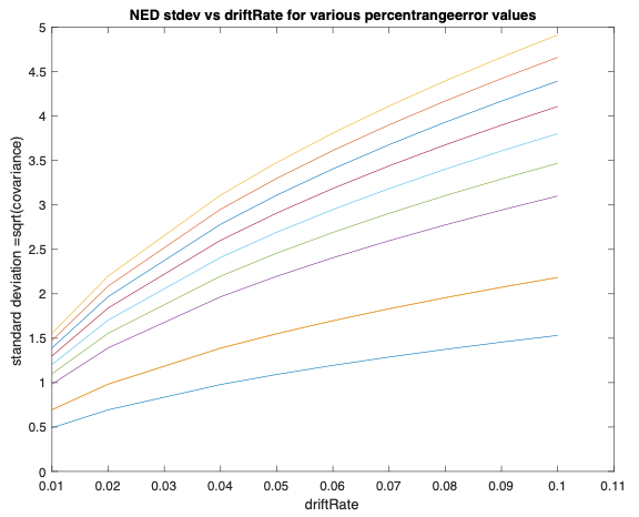
Fig 18: Predicted standard deviation of NE estimate using 11besms.
percentrangeerror = [.01 .02 .02 .04 .05 .06 .07 .08 .09 .10],. MNM = 2
Theory vs Practice and PF Modifications
An overview of how a particle filter works was described in "Summary of PF Operation". A detailed development is presented in Ref:Thrun, and its application to the AUV TRN problem is presented in Ref: Meduna. Presented here is a discussion of common practice for dealing with some issues that arise due to the difference between theory and practice when using a PF in the field. Also summarized are several additions to the basic PF algorithm that have been incorporated to improve its robustness.
The issues: unknown parameters, correlation and oblivious filters
The implicit assumption in any KF or EKF is that process noise (AHRS motion updates) and the measurement noise (beam lengths) are all zero mean Gaussian with known covariance and uncorrelated. It is also assumed and that all the parameters which define the measurements and equations of motion are known exactly. If these conditions are not met, the estimated values of NED and its covariance will be in error. Incorrect parameter values will bias the NED estimate. Correlated data will cause the filter to “over converge”, meaning that the estimate of uncertainty will be too tight. As stated above, this can cause a bad estimate of location to be accepted by the vehicle’s control system.
Clearly, it is unlikely that any fielded estimator will meet all these conditions.
Alignment biases (and other known types of sensor biases and drifts) will always exist. One “proper” way to deal with them is to include them as additional parameters to be identified along with the NED states of the system. Meduna provides examples of this for a wide range of sensor error in Ref:Meduna, but those capabilities have not been used in any field trials to date. One issue with augmenting the state vector is the computational cost. increasing the number of states greatly increases the number of particles required in a PF to maintain the same level of precision and may require reducing the number of particles used.
Correlation in the data will also exist and can be due to several potential sources. One is that measurements taken at one location can any information about the measurement taken at another location. Overlapping beam footprints are an obvious problem. A more subtle reason is that the terrain is assumed to be completely uncorrelated (completely random), which is not the case. Another source of correlation could be in how the beam data are filtered for noise and outliers. If a beam’s neighbors are used in the filtering, that is a potential source of correlation.
In practice, ensuring beam footprints are spaced at least 3 or 4 m apart in typical terrain helps reduce measurement correlation. Correlation can also be mitigated augmenting the state vector with coloring filters that describe the correlation (if it is known). Again, this results in an increase in the number of states.
A third issue when working with all types of Kalman filters is the “oblivious filter”. An oblivious filter exists when the process noise is too small. This causes the filter to assume that the process update is perfectly correct and hence measurements are no longer needed to correct the estimate. This can be a numerical issue.
Common practice in the field to deal with all these issues is to adjust the process noise artificially to achieve reasonable covariance values of the NED state estimate. If the unknown parameters are “small” and the correlation is not extreme this technique can work well.
Common practice: adjusting the process noise
Typically, the noise properties defined in the specification sheets for the sensors are “trusted” since they are often at least approximately correct. In the TRN code, the variable that defines the measurement noise is “percentrangeerror”. This is simply the assumed uncertainty in the beam length. It is implemented as a Gaussian covariance. A typical value is 4% of beam length.
The motion (process) noise is a different issue however. The disturbances acting on a system and the alignment of all the sensors are much more difficult to determine precisely. Further, they are often not Gaussian (e.g. alignment errors). Consequently, the process noise is often adjusted until credible covariances on the state (NED) estimates are achieved. (Adaptive process noise algorithms exist in the literature, but none is implemented in the current TRN algorithm.)
Two variables are used in the existing TRN code to describe process noise: the “driftRate” and the motion noise multiplier, “MNM”. driftRate is a bit of a misnomer. It is taken from the specification sheets for DVLs (e.g. 1% of distance travelled), but this is not a zero mean Gaussian error. This drift rate is typically associated with alignment errors and acts more like a bias in the motion.
In keeping with common practice, the TRN code approximates a Gaussian covariance to apply to the motion update which is large enough to account for the true motion uncertainty. The equation used in the TRN code is based on the circular error probability (CEP) calculations often used in projectile calculations. Here \(cep= driftRate * {\Delta}d\) and the standard deviation, \(\sigma\), is
\(\sigma = MNM * ({cep}\ /{\sqrt{-2*(log\ 1 - 0.5)}})\)
MNM is simply a convenient parameter used to adjust the amount of process noise in the calculations. It is currently defaulted to MNM = 2.
Note that other options for calculating the process noise standard deviation are available in the TRN code (e.g. a Gaussian noise added to a velocity input), but this formula has proven to be effective in previous field applications.
Additions for Robustness
In response to observed performance using TRN in the field, several additions to the algorithm have been incorporated to improve the algorithm’s robustness.
Normalized Innovations Sequence (NIS): It is possible for a PF to converge on a local minimum. When this occurs, the bounding box can tighten about the solution to the point that no particles are sampling the true location. To overcome this, the NIS logic was incorporated. This logic tests the innovations (difference between the measured and predicted beam lengths) for reasonableness. Specifically, it uses a chi-square test to determine the probability of observing a sequence of innovations. It the probability is low (e.g. less than 1%), it reinitializes the filter. See refHouts.
Alpha: TRN’s ability to produce an NED estimate depends on the information content of the terrain. If the terrain is flat, no information is present, but TRN may succeed in converging on a peak in the noise. To overcome this, an algorithm was introduced to reduce and broaden the PDF of the particle weights based on a measure of the variability in the terrain keeping the uncertainty of the estimate low. Alpha is the parameter that defines the reduction profile. See refDektor
Subsampling: For the baseline PF to function properly, ever beam from every particle must strike a point on the map. However, instances exist where the beam may land off the edge of the map or in a hole in the map. The subsampling algorithm was added to provide a proper calculation of the covariance update using only the subset of beams having valid measurements. See refStonestrom
Summary of EKF equations
where \(\frac{ \delta L_i}{\delta N}\) describes the change in \(i^{th}\) beam length for a small motion in the Northings direction, etc.
The process noise, \(\left[ \begin{array}{c} w_{\Delta N} \\ w_{\Delta E} \\ w_{\Delta D} \end{array} \right]_{n}\), is assumed to be zero mean, Gaussian with covariance
where \(\sigma_{\Delta D}\) is a constant (e.g. 0.5m and) \(\sigma_{\Delta N}\) and \(\sigma_{\Delta E}\) are computed from the Rayleigh distribution typically use in circular error probability (\(cep\)) calculations. Here \(cep\) is defined as \(cep = driftRate * \Delta d\) where \(\Delta d\) is the distance travelled in a time step, and MNM is the motion noise multiplier. The corresponding standard deviation is then
\(\sigma_{\Delta N} = MNM * (cep / \sqrt{(-2 * (log(1 - 0.5)))} \ )\)
The measurement noise, \(\left[ \begin{array}{c} v_1 \\ \bf{ .} \\ \bf{.} \\ v_m \end{array} \right]\), is assumed to be zero mean, Gaussian with covariance
where \(\sigma_{vi} = percentrangeerror * L_i\).
These equations can be written as
where the states, \(\bf{x}\), input, \(\bf{u}\) and output \(\bf{y}\) are
Given these equations, the basic operation of an EKF is an iteration between a process (or motion) update step and a measurement step. In the process update, the measured motions (u) are applied to the best estimate of the state (\(\hat{x})\) to yield an estimate of the state at the next time step (\(\bar{x}\)). An estimate of the covariance (i.e. uncertainty) of the state is updated from the current best estimate (P) to an estimate of what it will be at the next time step (M).
Process update
In the measurement update, the state estimate,\(\bar{x}\), is corrected using the measurement innovations, \(y- H \bar{ \bf{x} }_n\), to create the new best estimate of the state, \(\hat{x}\). The gain \(K\) determines how much the motion equations are to be trusted against the measurement equations. The gain \(K = P H^T {R_v}^{-1}\) is the optimal, time varying gain based on the noise parameters and is referred to as the Kalman gain. The prediction of the state covariance matrix, \(M\) is also updated to the new best estimate, \(P\), using the measurement information.
Measurement update
where \(K = P H^T {R_v}^{-1}\)
Note that this iterative process converges to a steady-state solution in which the amount of uncertainty introduced by the process noise is exactly offset by the information provided by the measurements.